Using Analog-Based Seasonal Weather Forecasts to Improve Grain Marketing Decisions

Introduction

Given the immense effect of weather on agriculture, skillful weather forecasts are important to agricultural producers for effective decision making. Weather forecasts affect operational decisions such as whether to irrigate (where applicable), when to apply fertilizer, when to spray herbicide and pesticide, and certainly the timing of planting and harvesting. At the seasonal time scale—say in the spring, just before planting—weather forecasts may be used for strategic decision making on outcomes, such as from preharvest hedging (hereafter referred to hedging), that will not be realized until the fall or harvest.

Historically, the lack of skill in generating seasonal weather forecasts has led the vast majority of agricultural producers to lack confidence to include seasonal weather forecasts in the hedging decision. Scientific advancements improving skill and accuracy of seasonal weather forecasts in the twenty-first century have occurred due to better understanding of the interplay between atmosphere, land, and oceans and well as faster and more detailed computer analysis of weather and climate data (Benjamin et al, 2018). Yet the adoption of seasonal weather forecasts in decision making in the agricultural sector has remained low. According to Klemm and McPherson (2018), the lack of adoption of seasonal weather forecasts can be attributed due in part to a lack of stakeholder relevance of the forecast information, a lack of forecast accuracy, or simply because the forecasts are too difficult to understand. The goal of this paper is to motivate the use of a modern seasonal weather forecast in the hedging decision. We achieve this goal by investigating how modern seasonal weather forecasts are established and develop a simple hedging model based on the seasonal weather forecast.

Perhaps the primary issue with the traditional seasonal weather forecast is the manner in which it has typically been communicated to users. For example, seasonal outlooks issued by the National Oceanic and Administration (NOAA) Climate Prediction Center (CPC) only show probabilities for above- or below-average temperatures and precipitation and where there is simply an “equal chance” for either outcome. This approach averages forecasts over one or three months, does not give insights about the expected magnitude of anomalies,¹  and does not provide any information about when anomalies of temperature and precipitation are most pronounced, leaving agricultural decision makers with little actionable information.

In our approach to seasonal weather forecasting, we rely on analog years, which are simply years in the past with weather patterns similar to those projected by the weather models for the summer growing months of June, July, and August. In practice, a given year generally has three to five analogs. The benefit of having multiple analog years is twofold: It can narrow the range of likely outcomes in the coming season and it can give early warning to the possibility of a significant deviation (positive or negative) from trend in the coming season. For example, two of the three analog years from Atmospheric and Environmental Research, Inc. (AER) for 2012 had droughts over large portions of the Corn Belt. This would have provided a useful early warning to the developing flash drought in 2012 (Basara et al., 2019) for a producer engaging in hedging. A flash drought is defined as a rapid onset and intensification of drought characterized by abnormally high temperatures, increased wind speeds, greater incoming solar radiation, and rapid depletion of soil moisture that leads to a marked decline in vegetation health (Otkin et al. 2018). Relating forecast information to analog years can give agricultural producers more context about the forecast information through yields experienced in analog years.

One of the most financially important decisions producers make is when to hedge a crop and how much crop to hedge (McKinnon, 1967; Chavas and Pope 1982; Pennings and Meulenberg 1997). The purpose of hedging is to reduce price risk exposure, but hedging in the preharvest environment becomes more complicated as the crop is yet to be produced. Reducing price risk through preharvest hedging must be tempered with the possibility of buyback, when contracted bushels exceeds produced bushels and fall prices are higher than spring prices (McKinnon, 1967). We demonstrate how incorporating a seasonal weather forecast using analog years can lower the probability of buyback for the hedger. For the traditional nonhedger, lowering the probability of buyback helps incentivize hedging. We demonstrate our approach by presenting the results of a study in which analogs from an AER February seasonal outlook were used to forecast the deviation from the U.S. national corn yield trend for the upcoming season.

Methodology and Data Sources

To generate an expected yield, we start out by using historic U.S. Department of Agriculture (USDA) data of observed U.S. corn yield to calculate a 50-year trend line (1969–2018). We then calculate the percentage deviation from the trend for each year. Yield predictions for upcoming seasons were then created based upon the outcomes in the analog years. The better the yield outcomes in the analog years, the greater the percentage deviation above trend; the worse the season, the greater the percentage deviation below trend. Using this approach, we calculated the upcoming growing season forecast for the years 2001–2018 from past early spring analogs that were produced by AER (labeled by the blue bar called “Forecast,” Figure 2). Those forecasted percentage deviations from trend were compared to the actual percentage deviations from trend (labeled by the red bar called “Actual,” Figure 2).

Figure 1. Temperature (degrees F) and
precipitation (in.) departures at Ames, Iowa,
1991–2020

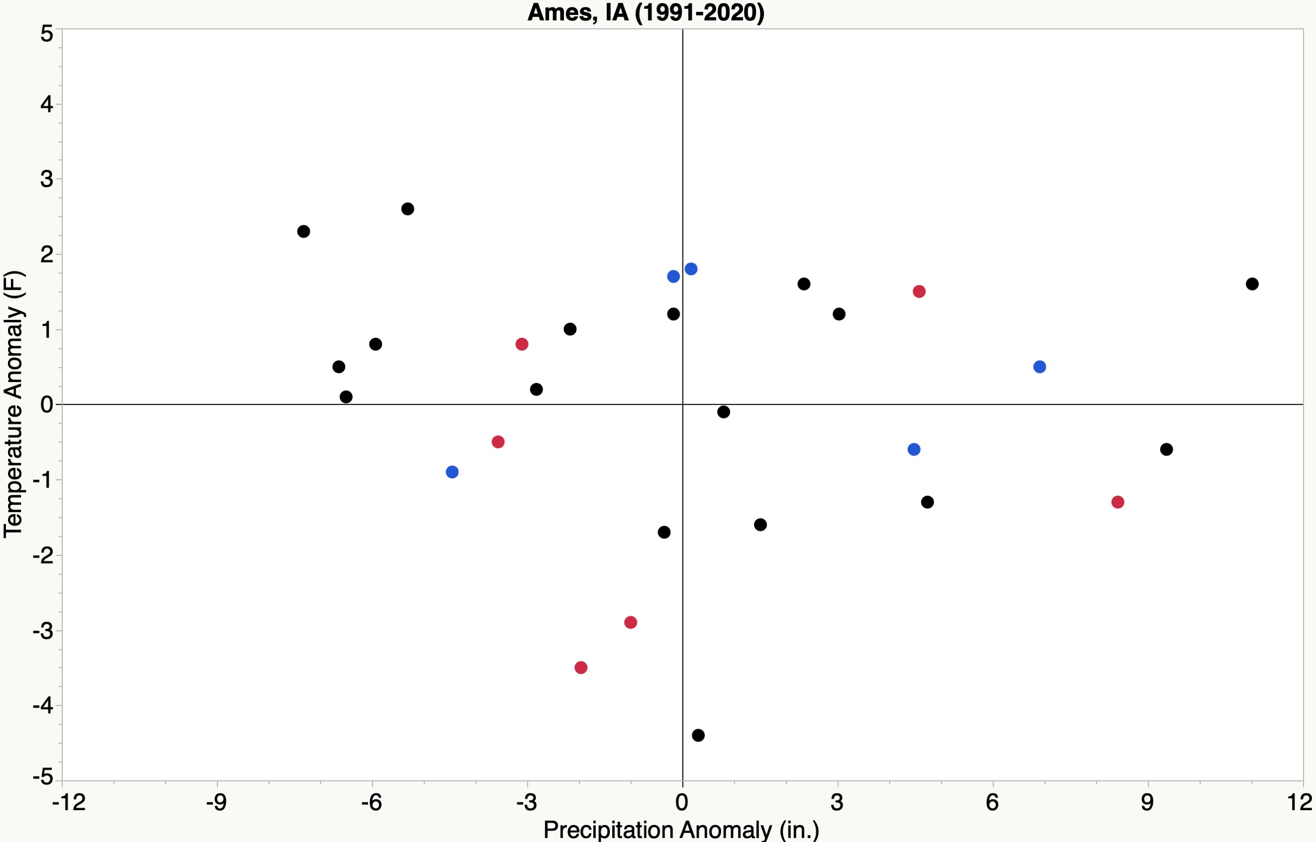
Notes: The figure excludes 1993 and 2010, which were
significant wet outliers. The red (blue) dots represent a
season with El Nino (La Nina) conditions during the
summer months (June–August).

---

Figure 2. December Corn Futures Spring
Price (Red Circle) and Fall Price (Black
Cross) across Time

---

Figure 3. Projected Percentage Deviation
from Trend on Corn Using the Analogs (Blue
Bars) versus Actual Percentage Deviation
from Trend on Corn (Red Bars)

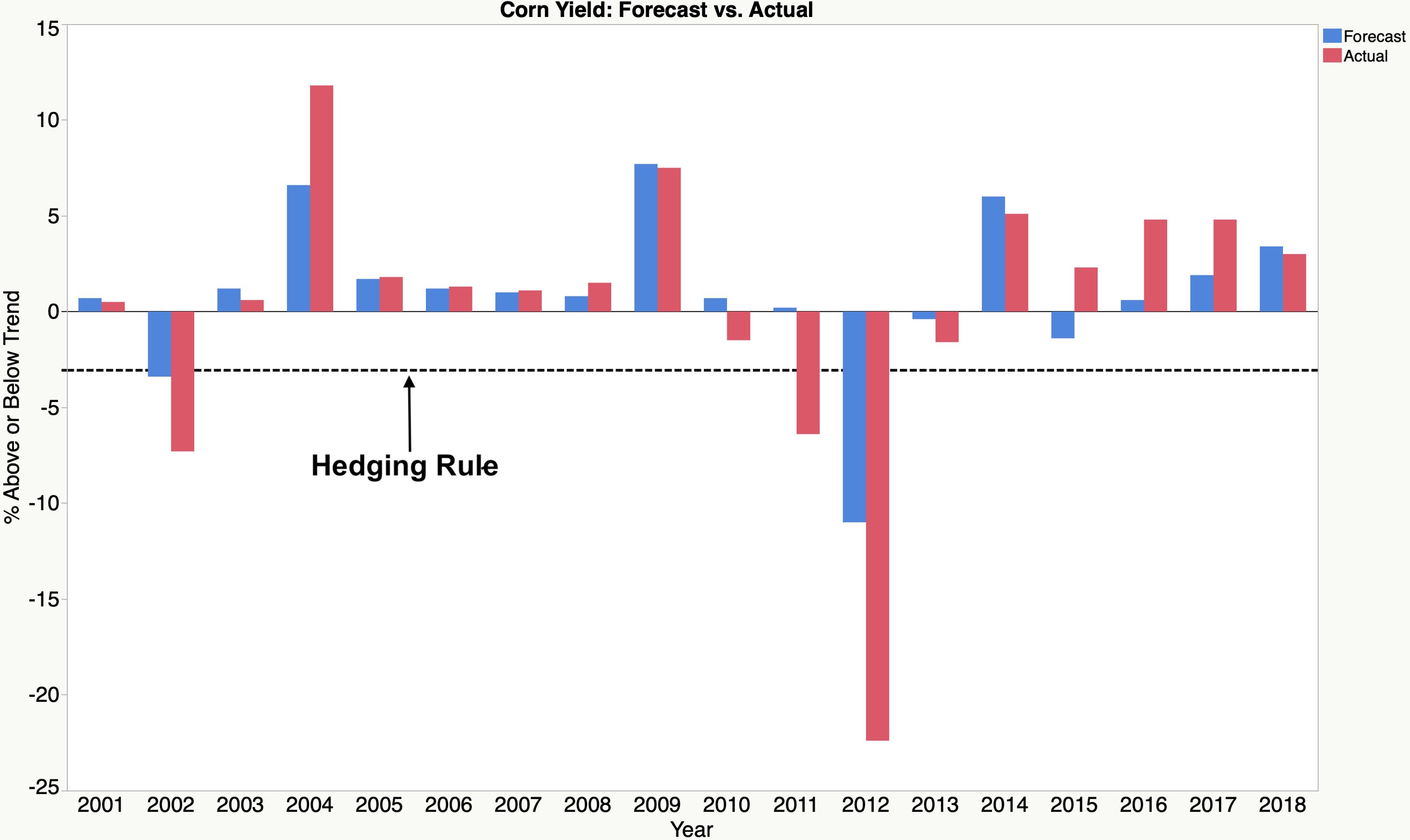
Notes: The line at 3% below trend marks the value at which a
producer would opt to not hedge, leaving all production to be
sold at harvest.

---

Figure 4. Comparison of Net Revenue
between Hedging (sell 60% of grain in the
spring) and No Hedging (sell 100% of grain
in the fall)

Notes: The hedging rule was set by the analog-based forecast.

The AER analog model uses comprehensive set of inputs to generate a forecast of temperature and precipitation anomalies for the United States. Inputs include but are not limited to the El Niño Southern Oscillation (ENSO), surface and oceanic temperature trends, snow cover from remote parts of the world, and the North Atlantic Oscillation (NAO) and Arctic Oscillation (AO) patterns. The inputs are then used in a statistical pattern-matching algorithm that uses machine learning to guide the selection of analog years. The analog years for the coming season are given each year in the AER February crop outlook, which is freely available on the AER website (https://www.aer.com ). An archive of past analogs (2001–present) can also be found on the AER website.²

Producers can also use climate data and the ENSO Index from the CPC to get a better idea of what type of weather or conditions an analog(s) represents. An example of an application of these data are shown in Figure 1, where the dots represent the anomalies of temperature and precipitation over the past thirty summer seasons at Ames, Iowa. The red (blue) dots represent summers where El Niño (La Niña) was present, with El Niño being more common in seasons that were cooler and drier than average (lower left quadrant) and La Niña being more prominent in seasons that were warmer than average.

A Simple Hedging Rule

We construct a simple hedging rule that relies on the weather forecast to decide whether to engage in hedging. The hedging rule contains two important elements and can be modified by the user. First, we sell only a percentage of expected production. Leaving crop to be sold at the harvest price provides protection from unforeseen events while also providing a reasonable amount of grain sold, thereby protecting farm income from price declines. Second, the hedge decision is based upon the percent change in U.S. corn yield from trend. This feature allows for the user to determine when they would engage in hedging. Our simple hedging rule is designed to limit the probability of buyback at high prices, which by design provides the highest probability of selling at the higher fall prices in drought years.³  An example base hedging rule: If the forecasted deviation of the U.S. corn trend was higher than 3% below trend (–3%), sell 60% of corn at the spring price (SP), otherwise sell 100% of corn at the fall price (FP).⁴  We applied a $0.10/bu cost to hedge and an additional $0.10/bu cost to buyback when in an oversold position.⁵  December prices obtained from the Chicago Board of Trade (CBOT) and are graphed in Figure 2. We calculated per acre net revenue from hedging using the following formula in years i the hedging rule applies, that is when the U.S. corn yield was projected to be higher than 3% below trend: (spring price × 0.6 × expected yield) + (fall price × (1 – 0.60) × (expected yield – harvested yield)) – hedging cost – buyback.⁶  The expected yield in this case is simply the corn yield at trend for a given year. Per acre revenue with no hedging was calculated as: fall price × harvested YIELd. We compare outcomes from our simple hedging rule to a producer selling everything at harvest and to a producer who always engages in hedging each year during the spring before April 1.⁷

Results

The median of the AER analogs produced useful yield projections, correctly projecting the direction (higher or lower from expected yield) of the final yield in 15 out of 18 years (Figure 3). Of the 15 correct projections, the AER analog model was also able to correctly predict the major drought year of 2012. This is especially important as drought years cause prices to rise, thereby lowering the effectiveness of hedging. For the three years during which the AER analog model did not correctly identify the direction of the corn trend, the AER estimated deviations from trend were minimal. With a small AER deviation from trend, it is not surprising that the direction of the final yield deviation was incorrect. Put another way, the AER analog model was able to correctly predict the direction of large deviations in final yields. The AER analog model appeared to be working as intended, to protect producers from hedging when droughts are forecasted and promote hedging when yields are expected to be much better than expected. Because the AER analog model correctly predicted future droughts, the probability of buyback fees appears to be limited.

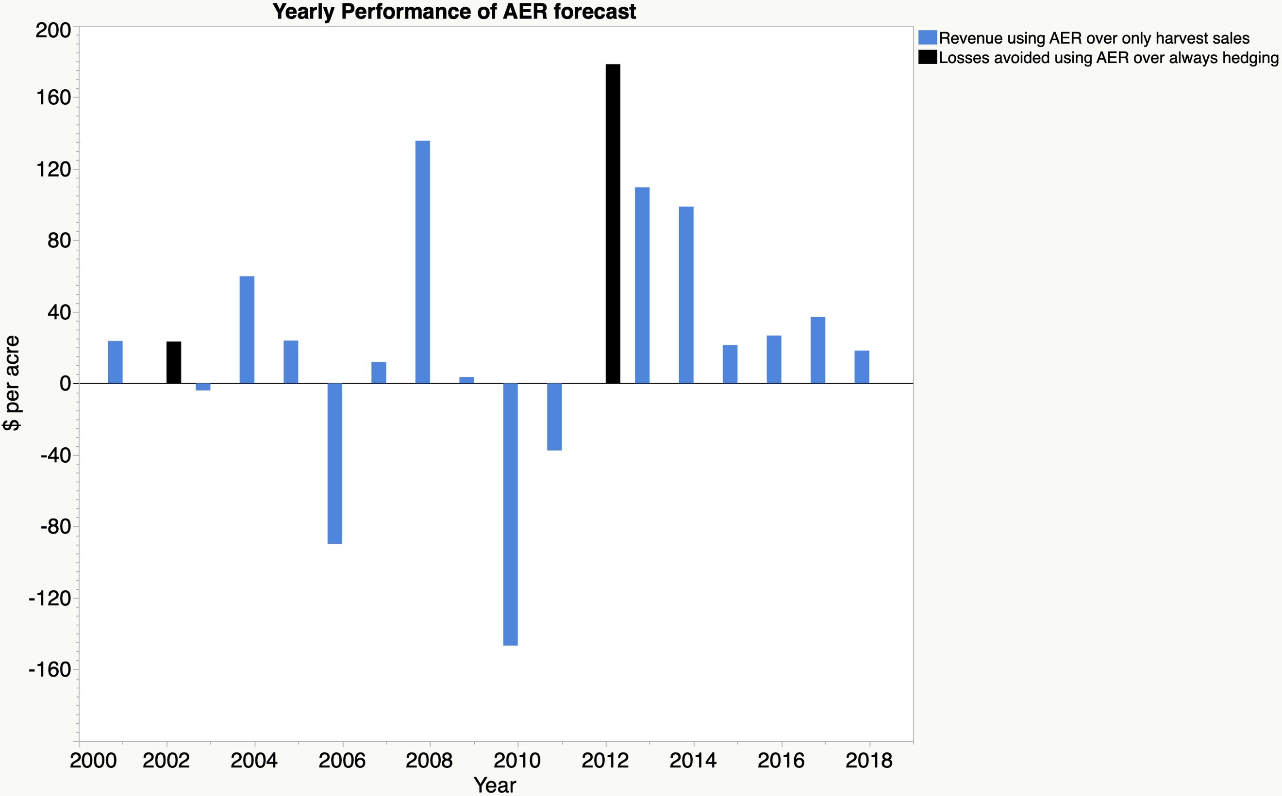
For results from the simple hedging rule, we begin by discussing results when compared to someone who is a 100% harvest time seller. We follow this discussion by comparing the results to a producer who always engages in hedging, no matter the year. Results suggest that by incorporating strategic hedging (through the inclusion of the weather analogs) into the decision framework when no hedging existed before, the producer would have gained an additional $16.28/acre on average (Figure 4, blue bars). However, in order to achieve the average, the hedger must financially survive the yearly financial variations. Yearly financial variations in results still exist in each year as the fall price is not only influenced by supply but also demand. In the years where hedging occurred, the hedger gained in 12 out of 16 years, with the highest gain of $135.72/acre in 2013 and the largest loss of $146.70/acre in 2010. Recall that the strategic hedging model did not expose the traditional, nonhedging producer to costs associated with hedging in the drought year of 2012.

We now turn our comparison to someone who always engages in hedging. In this case we are interested in the value of losses avoided from not hedging when a drought occurs (Figure 4, black bars). On average, a producer who engages in strategic hedging improves revenue by $11.22/acre over someone who always hedges. The difference comes from not engaging in hedging when a drought is forecasted. For the 2012 drought, the AER analog model suggested no hedging, saving the producer $178.56/acre as a result. During a smaller drought in 2002, the AER analog model saved the producer $23.40/acre.

These results suggest the AER analogs model, along with the hedging decision criteria, can improve the financial performance from hedging. The improvement comes in two forms. First, the hedger is less likely to be hedged during a drought year. This is an important outcome for both the traditional hedger and for producers who do not engage in hedging. Second, the hedger has price protection in years when the spring price is substantially higher than the harvest price. This is important for the nonhedger as they are passing up higher revenues generated from hedging. However, our results do not make hedging following the AER analog model perfect, as there were years when the harvest price turned out to be higher than the spring price (2006 and 2010). The AER analog model along with the simple hedging decision criteria, on average improves the financial outcome from strategic hedging.

Discussion

In this article, we investigated the role of adopting the AER analog-based seasonal weather forecast and a simple preharvest hedging decision rule to evaluate farm financial outcomes. Results indicate that the AER analog-based seasonal weather forecast model and the simple hedging decision rule provided financial benefits for both producers who traditionally sell everything at harvest and for producers who traditionally hedge every season. The traditional nonhedger would have received an additional $16.28/acre on average and surviving years where buyback exists. This is where the AER analog-based model performed well, as it avoided both buyback costs and hedging costs as the model suggested no hedging in the drought of 2012. The traditional hedger also avoids buyback by avoiding hedging in drought years, thereby improving financial performance by $11.22/acre on average.

Forecasting a drought or other regional hydrometeorological extremes several months in advance is difficult; these extremes may not be easily detectable in a summer forecast that is issued the previous late winter or early spring. However, using analog years in conjunction with a grain marketing plan appears to provide a greater likelihood of early warning of an impending drought. For example, the analogs used in this study were able to show an increased likelihood of drought in 2002 and 2012. In both years a farmer would have financially benefitted from following the AER analog forecast and simple marketing plan.

This evaluation provides a framework on how to combine an analog based forecast with a hedging model to improve farm financial performance. Our approach is straightforward and perhaps overly simple.  Our framework can be applied to the upcoming crop year by evaluating the AER seasonal weather forecast and applying this information to your marketing plan.⁸ 

We do, however, want to note a few limitations with this approach. First, while the use of analogs was broadly successful for this study, this was only applied to corn and might not be applicable to other crops. Second, the net revenue per acre values from this study were calculated in a very simple manner and thus may likely underestimate performance from other, more sophisticated techniques. Third, we do not consider the role of basis risk.  There could be events where cash and futures prices diverge, thereby lowering the effectiveness of the hedge. Fourth, this method also does not account for related farm risk management tools, like crop insurance. Given the large number of available crop insurance contracts, we plan on investigating the role of crop insurance in future work. Fifth, though the analogs were produced in February of every year from 2001 to 2018 at AER, the study was conducted as a hindcast, and past success is not a guarantee of future success (Milly et al., 2008). Given that AER produces monthly forecasts, the hedging decision criteria can be improved upon by evaluating the subsequent month’s forecast. If hedges were placed early due to no drought being forecasted and then a drought emerges, hedges could be removed before prices start to rise. The alternative could also happen. Developing a dynamic hedging model that adapts to new information would likely improve performance.

Overall, the results of this study demonstrate an advantage of simultaneously applying a forecasting model and grain marketing plan. We found evidence of additional financial benefit in using analogs as part of a corn marketing plan, as they can help indicate whether corn farmers should hedge.

For More Information

Basara, J.B., J. Christian, R. Wakefield, J. Otkin, E. Hunt, and D. Brown. 2019. “The Evolution, Propagation, and Spread of Flash Drought in the Central United States during 2012.” Environmental Research Letters 14: 084025.

Benjamin, S.G., J.M. Brown, G. Brunet, P. Lynch, K. Saito, and T.W. Schlatter. 2018. “100 Years of Progress in Forecasting and NWP Applications.” Meteoological. Monographs 59(1): 13.1–13.67.

Chavas, J.P., and R. Pope. 1982. “Hedging and Production Decisions under a Linear Mean-Variance Preference Function.” Western Journal of Agricultural Economics 7(1): 99–110.

Klemm, T., and R.A. McPherson. 2018. “Assessing Decision Timing and Seasonal Climate Forecast Needs of Winter Wheat Producers in the South-Central United States.” Journal of Applied Meteorology and Climatology 57(9): 2129–2140.

McKinnon, R.I. 1967. “Futures Markets, Buffer Stocks, and Income Stability for Primary Producers.” Journal of Political Economy 75(6): 844–861.

Milly, P.C.D., J.L. Betancourt, M. Falkenmark, R.M. Hirsch, Z.W. Kundzewicz, D.P. Lettenmaier, and R.J. Stouffer. 2008. “Stationarity Is Dead - Whither Water Management?” Science 319(5863): 573–574.

Otkin, J.A., M. Svoboda, E.D. Hunt, T.W. Ford, M.C. Anderson, C. Hain, and J.B. Basara. 2018. “Flash Droughts: A Review and Assessment of the Challenges Imposed by Rapid-Onset Droughts in the United States.” Bulletin of the American Meteorological Society 99: 911–919.

Pennings, J.M., and M.T. Meulenberg. 1997. “Hedging Efficiency: A Futures Exchange Management Approach.” Journal of Futures Markets: Futures, Options, and Other Derivative Products 17(5): 599–615.