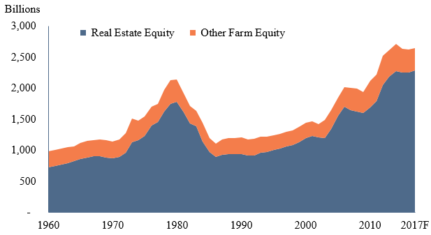
A rising interest rate environment has far-reaching implications for America’s farmers and ranchers. Higher interest rates could impact farmers’ income statements by affecting commodity prices and interest expenses (Henderson, 2018; Kuhns and Patrick, 2018). Increasing interest rates are also likely to impact farmers’ balance sheets by impacting the market value of both their assets and liabilities. The USDA currently projects that farm sector debt has increased by more than 30% over the last decade, even after adjusting for inflation. But farm asset values have also grown and the farm sector, in aggregate, still has relatively low leverage, with debt accounting for only 13% of asset values. This has left farmers with a record $2.7 trillion in equity at the end of 2017 according to current USDA projections (ERS, 2017), most of which is held in farm real estate (Figure 1). If farm assets decline in value or farm debt rises more quickly than assets, farm equity is eroded and, with it, the hard work and savings of millions of farmers and ranchers. Since the market value of assets and liabilities is affected by interest rate fluctuations, farm equity is also sensitive to interest rate changes.
Analysis of the interest rate risk inherent in farmers’ balance sheets has often focused on the direct impact of interest rate changes on asset values. Long-run interest rates have been used to proxy farmland capitalization rates, and rising rates could reduce the land values supported by current income levels (Schnitkey and Sherrick, 2011). Rising interest rates can also have a direct impact on the value of farmers stored commodity inventories by reducing the value of their future revenue streams (Henderson, 2018). While often not explicitly specified, these types of analyses are related to the financial concept of duration, which is often used in financial analysis to measure the average timing of a stream of cash flows. Modified duration can be used to gauge a financial instrument’s sensitivity to interest rate movements. Differences between the timing the cash flows associated with farmers’ assets and liabilities, often referred to as a duration gap, can also expose farmers’ balance sheets to interest rate risk.
This article illustrates how duration can be applied to farmers’ balance sheets. After illustrating their application, the concepts are used to measure the farm sector’s duration gap or the difference between the timing of the cash flows associated with the sector’s assets and liabilities. Since equity is the difference between assets and liabilities, this analysis can be used to determine how the equity in farm operations is impacted by changes in interest rates. The sections below outline the basics of financial duration, demonstrate how a single balance sheet is affected by changing interest rates, and then apply these concepts to at the U.S. level to show how farm sector equity may be impacted by changes in interest rates. Practical implications of the exposure to interest rate risk are provided along with guidance for managing the risk exposure for farm businesses.
In finance, an asset’s value is often expressed as the sum of the present value of its future cash flows. Duration is used to provide a measure of the timing of cash flows associated with a given financial instrument (Macaulay, 1938). When calculating duration, the timing of each cash flow is weighted by the size of the present value of that cash flow relative to the present value of all cash flows:
(1) Because duration considers the timing and size of cash flows as well as the discount rate used to calculate the present value of future cash flows, it can be thought of as measuring the weighted average timing of the cash flows generated by a given asset or liability. Short-term assets and liabilities have lower duration values because cash flows happen over a short period, whereas long-term assets and liabilities have higher duration values because cash flows are more spread out over a longer period.
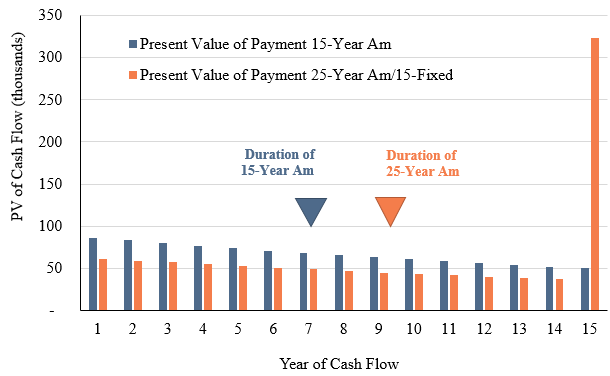
Applying duration to the cash flows associated with a farm operation’s debt provides a way to measure the average timing of cash flows due from a given liability. For example, a farm-operating loan with a single payment due in 12 months would have a duration of 1.0 year. On the other hand, a 15-year fixed rate farm real estate loan has an approximate duration of 9.5 years if the payments do not vary during the life of either debt. Even if two loans have the same term, they may not have the same duration if there are differences in the size or timing of payments. Figure 2 demonstrates this concept by calculating the duration of two long-term real estate loans, each with a term of 15 years. The first loan is fully paid off at the end of the 15-year term (typically referred to as being fully amortizing), while the second has a 25-year amortization period. The balance remaining after the 15-year term is due as a balloon payment. Although the loans have the same 15-year term, the loan with the balloon payment has more cash flow weighted in later years and thus has a longer duration.
Compared to calculating the duration of farm debt, where the timing of cash flows is often known, the application of duration to farmers’ assets can require careful consideration of the underlying cash flows. Once the timing of cash flows is determined, the same analysis can also be applied to a farm operation’s assets to understand the average timing of the cash inflows they generate. For example, farmland can generate cash flows in the form of annual lease payments, or the sale of crops and livestock can generate cash flows in the form of one-time cash payments.
While understanding the timing of cash flows provides useful information on financial instruments, the idea of duration has been extended to provide an indication of the instrument’s interest rate sensitivity. Modified duration provides a useful extension of duration that measures the change in the value of an asset resulting from a change in market interest rates (Redington, 1952). Modified duration is the change in the value of an asset or liability given a change in market interest rates. For example, if a farm loan had a modified duration of 1.5, a 1-percentage point increase in interest rates would cause a 1.5% decrease in the value of the loan. This interpretation of modified duration is incredibly powerful: In one number, an analyst, portfolio manager, banker, agricultural lender, or farmer can measure exactly how much interest rate risk exists on any asset or liability. The higher the number, the greater the change in the value of the asset or liability in response to movements in market interest rates and therefore, the greater the interest rate risk:
(2)  (3)
(3)  Both assets and liabilities are exposed to changes in interest rates. Falling interest rates lead both asset and liability market values to rise by increasing the present value of associated cash flows, while rising interest rates decrease the present value of future cash flows, causing the market value of asset and liability values to decline. For a farmer, the expected rise in interest rates will cause the market value of assets and debt to fall, all else equal. Whether the market value of a farmer’s equity rises or falls with interest rates depends on the relative sensitivity of assets and debt. However, the market value of equity must be exposed to interest rate risk since it is the difference between assets and liabilities and each is exposed to interest rate risk.
Since modified duration measures this sensitivity, the weighted difference between the modified duration of assets and liabilities, typically referred to as the duration gap, can be used to measure the sensitivity of equity to interest rate fluctuations:
(4)  Once calculated, the duration gap can be combined with a farmer’s current asset position and the interest rate change to determine the movement in equity:
(5)  If assets have a longer duration than liabilities, the duration gap is positive, and the value of equity and a rising interest rate environment will reduce that value of equity. Conversely, if the debt has a longer duration, the duration gap will be negative, and a rising interest rate environment will increase that value of equity.
Duration gap analysis has been used extensively by the banking and insurance sectors for decades as a way to measure and manage portfolio interest rate risk (Bierwag and Kaufman, 1985). Taken one step further, portfolio managers can immunize their balance sheets from interest rate risk by selecting assets and debts that offset to a duration gap of zero (Redington, 1952). For perfectly immunized portfolios, interest rates can go up and down and the value of the equity in the portfolio will not budge because any changes to asset values will be perfectly offset by changes in the value of liabilities. Applying the analysis to the farm sector highlights the inherent interest rate risk in the farm sector’s balance sheet from differences in the duration between farmers’ assets and liabilities.
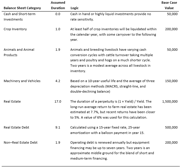
To simplify the calculations, the farm balance sheet has been broken up into seven categories, each with a defined duration value (see Table 1). Most assets and debt categories have relatively straightforward expected cash flows. The largest exception also happens to be the largest category, farm real estate. For demonstration purposes, this analysis treats farm real estate as a perpetuity that pays an annual yield of 6%, which is in line with USDA estimates (ERS, 2017). A perpetual average return of 6% implies a duration of 17 years.
Table 1 also lays out a hypothetical cash grain operation in the Midwest with moderate levels of leverage. The values in Table 1 are like those from the USDA’s 2016 Agricultural Resource Management Survey (ARMS) but with slightly more debt to better illustrate the effects of duration analysis. The hypothetical operation has very low levels of cash and animal inventory and has more of its assets in either crops in the bin or in the ground, as well as in machinery and land. Approximately 75% of this operation’s assets are in the value of farm real estate, a level that mimics the overall sector. On the other side of the balance sheet, the operation has a real estate loan with a 33% loan-to-value and an operating line that mirrors the value of crop for marketing. Weighting the durations by the balance sheet values, the assets have an average duration of 13.5 and the liabilities have an average duration of 7.1. Given the weight of assets and liabilities on the balance sheet, this leaves a duration gap of 11.0. The duration gap implies that a 100-basis point increase in underlying interest rates will decrease the value of equity by 11% of assets, resulting in a loss of roughly $215,000.
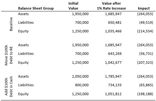
What is the farm operation to do about this erosion of equity? Immunization theory provides a few simple options. The operation could extend the repayment period on their loans to extend the duration of liabilities. Table 2 compares a pair of alternatives for minimizing the impact of rising rates on the operation’s equity value to the baseline scenario. The operation could use a strategy that merely affects the length of the leverage rather than the overall amount of leverage in the firm. By simply lengthening the duration of liabilities by refinancing $100,000 of debt into the longer-term real estate loan, the operation can protect $8,000 of its equity from interest rate risk. Another option is for the operation to increase its leverage and change the composition of its assets to shorten their average duration. For example, the firm could take out an additional $100,000 on the long-term loan and use the proceeds to increase their working capital by investing in short-term assets or cash. Holding more short-term cash assets would allow the operation to add liquidity to the balance sheet and reduce the duration gap by shortening the average duration of assets and increasing the average duration of liabilities. In turn, the operation can protect nearly $20,000 of its equity from interest rate risk.
Importantly, in this example it is virtually impossible for this farm to fully immunize the balance sheet from interest rate risk due to the relatively high duration of farm real estate. Financial institutions often overlay off-balance sheet derivatives such as interest rate futures or swap contracts to tighten the duration gap (Bierwag and Fooladi, 2006). These complex financial instruments are often inaccessible to smaller farm operations, but they should be considered as a possible means of reducing interest rate risk. And while not all farm balance sheets can be fully immunized, any reduction in duration gap can protect equity from the tide of rising interest rates.
Interest rate risk presents itself in the aggregate farm sector balance sheet as well. By grouping the balance sheet items published by the USDA Economic Research Service into the same classifications used in the previous example, the assumed asset classification durations can be used to calculate the sector’s duration gap over time. Given that farm real estate assets have typically made up more than 70% of all farm assets, the long-term nature of farm real estate dominates the sector’s asset duration calculation. Since 1960, the average duration of farm assets is 13.4. Of note, there are periods with a slightly higher farm asset duration in the early 1980s and 2000s, when farm real estate assets were 80% of the balance sheet or higher. Since 1960, farm liabilities have averaged a duration of roughly 5.7, with higher periods in the 1980s and 2000s when farmers used a greater mix of long-term real estate financing.
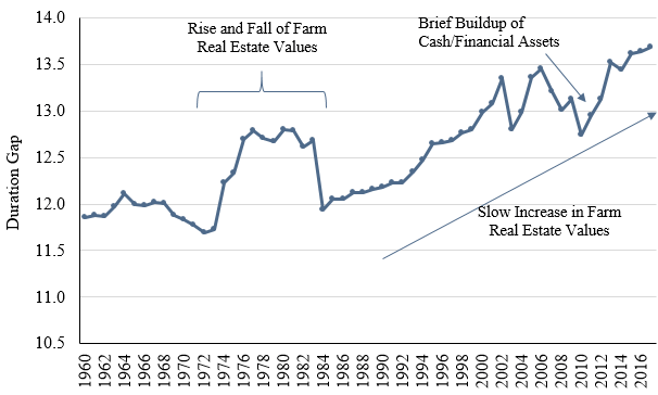
Figure 3 shows the calculated historical duration gap for the sector from 1960 through 2017. The gap has been gradually increasing as real estate has increased as a percentage of farm assets. Two periods stand out as opposing the slow drift: the boom and subsequent bust of the 1970s and 1980s and the years from 2008 to 2012, when high profit levels increased farm operators’ cash and short-term financial positions to record highs. In 2017, the farm balance sheet duration gap stands at 13.7; holding everything else constant, if rates rise by 1 percentage point, this analysis indicates farm equity would fall by $419 billion given the duration gap and initial $3 trillion asset base.
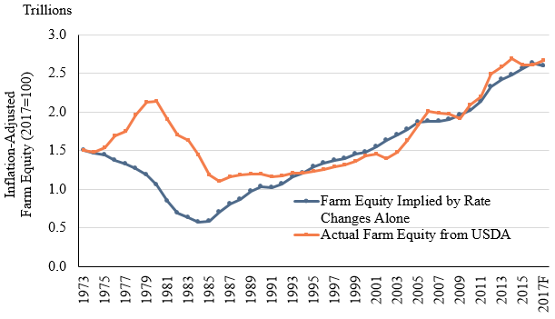
The duration-implied value of farm equity tracks the path of reported farm equity surprisingly well. The durations of all farm assets and liabilities is easily calculated from the values in Table 1. The implied change in equity from a given starting point is the duration gap multiplied by the level of change in interest rates. Using the annual difference between the 5-year moving average 10-year Constant Maturity Treasury rate as a proxy for yield curve shifts, rolling the implied value of farm assets and liabilities forward is a straightforward exercise. Figure 4 demonstrates the results of such an exercise, beginning with 1973 as a base year and letting farm equity float using only the duration gap and the change in interest rates from the prior year. The rapid rise in interest rates in the late 1970s implied a much deeper drop in farm equity than was experienced, but since 1990, the implied equity and reported equity have moved in near-lockstep. This relationship will be worth monitoring if the market yield curve continues to rise.
Understanding the balance sheet impacts of interest rate movements is the first step toward preparing for them. The value of future cash flows is affected by the level of interest rates, and asset and liability values are both functions of the value of cash flows. Since farmers’ asset and liability values are both sensitive to interest rate changes, farm equity is also affected by interest rate fluctuations. The scenarios outlined in this article illustrate how the long duration of farm real estate can make it difficult for the farm sector to eliminate its duration gap. Accordingly, farmers’ equity is adversely exposed to rising interest rates.
However, farm real estate may not be as interest rate sensitive as its duration suggests. Real estate is a natural inflation hedge, and rate sensitivity varies inversely with inflation sensitivity (Leibowitz, 1992). If interest rates increase in response to rising inflation, farm real estate values may not fall but instead rise, as home prices did in the 1970s. Second, landowners facing a sizable duration gap can always choose to lease out portions of their land holdings to shorten the duration of their portfolios. Leases have fixed time horizons with regular repricing, which gives the cash flows associated with the asset the ability to float with the market and thus the sensitivity to changes in market conditions and interest rates is greatly reduced. Finally, today’s lending marketplace offers more widely available and longer-duration loan products than were available during the 1980s. In this article, farm real estate debt was modeled assuming a 15-year fixed rate and 25-year amortization, but farmers have access to 20, 25, and even 30-year loan maturities. A 30-year fixed-rate loan has an approximate duration of 17.7, more generally in line with the land itself. Access to longer-duration debt capital could help protect farm equity in the event of rapidly rising interest rates.
Bierwag, G.O., and I.J. Fooladi. 2006. “Duration Analysis: An Historical Perspective.” Journal of Applied Finance 16(2):144–160.
Bierwag, G.O. and G.G. Kaufman. 1985. “Duration Gap for Financial Institutions.” Financial Analysts Journal 41(2):68–71.
Henderson, J. 2018. ”Monetary Policy and Agricultural Commodity Prices: It’s All Relative.” Choices 33(1).
Kuhns, R., and K. Patrick. 2018. “How Sensitive is Farm Sector Repayment Capacity to Rising Interest Rates and Farm Debt?” Choices 33(1).
Leibowitz, M.L. 1992. “A Look at Real Estate Duration.” In M.L. Leibowitz, F.J. Fabozzi, and W.F. Sharpe, ed. Investing: the Collected Works of Martin L. Leibowitz. Chicago, IL: Probus Professional Pub, pp. 461–480.
Macaulay, F.R. 1938. Some Theoretical Problems Suggested by the Movements of Interest Rates, Bond Yields and Stock Prices in the United States since 1856. Cambridge, MA: NBER Books.
Redington, F.M. 1952. “Review of the Principles of Life-Office Valuations.” Journal of the Institute of Actuaries 78(3):286–340.
Schnitkey, G.D., and B.J. Sherrick. 2011. “Income and Capitalization Rate Risk in Agricultural Real Estate Markets”. Choices 26(2): 1–7.
U.S. Department of Agriculture. 2017. USDA ERS Farm Balance Sheet Historical Data. Available online: https://data.ers.usda.gov/reports.aspx?ID=17835

