The pendulum of farm income has swung from record high levels at the beginning of the decade to an environment of extremely tight margins in 2016. U.S. Department of Agriculture (USDA) has forecasted nominal U.S. net farm and cash incomes to be the lowest levels in a decade. The net farm income levels are the lowest since 2002 (Figure 1). The declines reflect shrinking margins from declining crop prices and weaknesses in dairy and hog markets. The largest declines in net income are expected in the Corn Belt. According to the USDA Agricultural Resource Management Survey (ARMS) the average farm income for all farms in Kansas and Illinois more than doubled from 2005 to 2013 (Figure 2). However, net farm income levels in 2015 were negative for some individual producers. For example, in 2014 the average net farm income for the North Central Kansas Farm Management Association was $102,508 (KFMA, 2016). For 2015, the average net farm income for the same association was $11,452. It is also anticipated that average projected net farm income levels for 2016 are below levels to support family living and debt service for Kansas and Illinois producers.

Source: USDA-ERS, 2016b
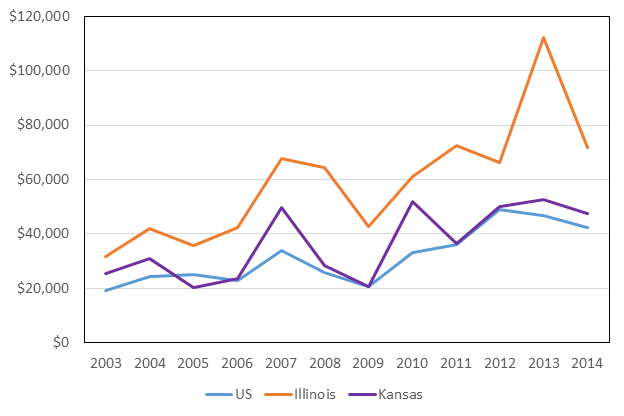
Source: USDA-ERS, 2016a.

Source: USDA-ERS, 2016a; FBFM, 2016;
KFMA, 2016.
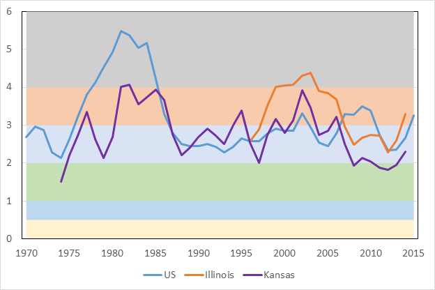
Economic downturns in agriculture increase the attention towards measuring financial stress in the sector and assessing the ability of producers to manage liquidity and debt. Production agriculture is characterized as using a low amount of debt relative to assets. The USDA forecasts a total farm debt of $373 billion in 2016, which is a 26% increase from 2011. Total assets in the farm sector are expected to exceed $2.82 trillion, resulting in a farm aggregate debt-to-asset ratio of 13.2%. Figure 3 reports the debt-to-asset ratio for the United States from 1970 to 2015 based on ARMS data, Illinois from 1996 to 2014 based on the Illinois Farm Business Farm Management Association (FBFM, 2016) data and Kansas from 1973 to 2014 based on the KFMA data. This commonly-used metric is often cited as a financial stress indicator and often interpreted as an indicator of the low leverage in the agricultural sector. Note the mean for farm businesses in Kansas and Illinois exceeded 30% in 2001 and 2002. Since then, it has generally declined to 19% in 2014; this is higher than the USDA all-farms industry average of 15% in 2002 and 13% in 2014.
A primary weakness in using this aggregate measure of financial condition is the omission of any distributional characteristics among agricultural producers. Since a high percentage of producers have little or no debt, the aggregate measure provides little evidence of the proportion of farms with high levels of financial leverage and financial risk. Figure 4 indicates the distribution of debt-to-asset ratios for Illinois and Kansas farms.
In general, the proportion of Illinois and Kansas farms with higher debt-to-asset ratios has declined over this 12-year time period, an indication of improved financial resiliency. But with current declining values of farmland, machinery and equipment, and grain and livestock inventories in the 2014-2016 period, the financial vulnerability of those farms with higher debt-to-asset ratios has increased. The distribution of debt-to-asset ratios in 2014 indicates that less than 2% of Illinois and Kansas farmers are vulnerable to financial failure—defined here as debt-to-asset ratios of 80% or greater—with only a modest decline in asset values; the proportion classified as vulnerable operators increases to 5% at the 60% debt-to-asset threshold.
The debt-to-asset ratio measure reflects solvency, that is, the risk-bearing ability. From a lender’s perspective it indicates the amount of secondary repayment capacity to service debt if assets are liquidated, or the financial reserves to support refinancing debt obligations if the borrower is unable to make debt servicing payments from cash flow or earnings. A common underwriting standard in agricultural lending is that the borrower should have at least as much at risk as the lender—that is, at least 50% equity in the business—to have adequate reserves to handle financial stress. The debt-to-asset distributions in Figure 4 indicate that 6.6% and 8.7% of the Kansas and Illinois farmers, respectively, would not meet this underwriting standard in 2014. With the decline in asset values and increased debt since that time, an even higher proportion are likely to encounter difficult conversations with their lender along with financial vulnerability.
The debt-to-asset measure of leverage is highly influenced by real estate values. Over 81% of assets in the agricultural sector are held in real estate that is valued on a market valuation basis. Farm real estate lacks liquidity and is characterized by low cash returns (Barry and Ellinger, 2012). Evidence from the residential real estate markets is that during a severe crisis, asset values experience larger than expected declines in market values. Although, there are no signs of a financial crisis in agriculture, changes in the debt-to-asset ratio will occur as land values adjust. Moreover, less than 10% of the assets held on farm balance sheets are highly liquid, meaning those other than real estate and machinery. Liquid assets and cash income are the primary sources of repayment for borrowers and are the drivers of the level of debt that can be serviced by agricultural producers. Hence, additional metrics beyond the debt-to-asset ratio could be used to enhance the assessment of financial stress in the agricultural sector.
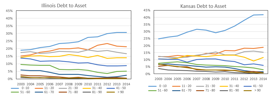
Source: FBFM, 2016 and KFMA, 2016
Working capital—current assets less current liabilities—is the first buffer borrowers can utilize in periods of cash shortfalls. Many agricultural producers improved working capital during the past decade. Working capital increased from an average of $179 per acre during the decade 1996 to 2006 to over $700 per acre in 2012 on Illinois Grain farms (Schnitkey, 2015c). The increase in working capital improved the overall liquidity of operations, but the improvement was muted by the increase in cash costs of production on grain farms during this same period. Non-land costs increased from $300 per acre to $615 per acre for corn from 2006 to 2013 (Schnitkey, 2015a).
The three primary reasons to hold liquid assets are for transaction purposes, to meet unforeseen cash shortfalls and to have flexibility for investment opportunities (Barry and Ellinger, 2012). Higher levels of operating costs require higher levels of liquidity for both transactions purposes and a buffer for potential downfalls. Moreover, the price of farm investment opportunities increased over this same period as well. The average level of working capital on Illinois farms could have purchased 50 acres of farmland in 2006. The average purchasing power level of working capital increased to 85 acres in 2012 and subsequently declined to 57 acres in 2014. Hence, the cash reserve buffer from increases in aggregate working capital is partially offset by the increased liquidity needed for transactions and investment opportunities.
A critical financial stress indicator for agriculture is the level of working capital relative to the working capital burn rate. Working capital burn is simply the projected net cash loss expected over the next year. The working capital expressed relative to the burn rate provides a measure of the number of years before working capital is exhausted. In Illinois, working capital change is projected at -$11 per acre for owned farmland, meaning that working capital would decrease $11 for each acre owned (Schnitkey, 2015b). On average, land that is cash rented has a projected -$121 per acre working capital change or burn and share rented land has a -$72 change.
Since the debt-to-asset ratio may not be an effective indicator of the level of debt that can be serviced by a farm borrower or an adequate metric of financial stress in the agricultural sector, the debt-servicing to income ratio is an alternative metric. It is a commonly-used metric for determining the level of debt a household can service as well as a primary underwriting standard in the housing sector. The level of debt for commercial loans is also typically driven by the ability to generate cash. The most common measure of leverage is Net Debt—debt less cash and equivalents—divided by Earnings Before Interest Taxes, Depreciation and Amortization (EBITDA). EBITDA is a commonly-used proxy for cash flow being generated by a business prior to debt service and income taxes.
Moody’s Corporation, the parent corporation of Moody’s Investor Services, provides credit ratings and research across alternative debt instruments including approximately 11,000 corporate issuers. Moody’s Investor Services publishes their rating methodology for companies in different market sectors. The published methodology is useful in understanding the qualitative and quantitative factors used by Moody’s in their credit rating process. Common rating factors used by Moody’s for corporate businesses include scale, business profile, profitability, leverage, financial policy, market position and business risk. The four methodologies are:
| Rating Category | Debt to EBITDA Ratio |
| AAA | 0 to 0.50 |
| AA | 0.51 to 1.00 |
| A | 1.01 to 2.00 |
| Baa | 2.01 to 3.00 |
| Ba | 3.01 to 4.00 |
| B | 4.01 to 6.00 |
| Caa | 6.01 to 8.00 |
| Ca | > 8.00 or < 0 |
Using farm-level data from the FBFM and the KFMA to evaluate distribution of farms by Debt to EBITDA, the Debt to EBITDA ratio is:
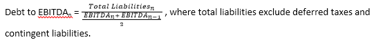
A two-year average of EBITDA is used to avoid larger annual swings in income. The Moody’s ratings cut-off values for Debt-to-EBITDA varied slightly across the four methodologies. The values used for this analysis are provided in Table 1. In general, a rating of B or below is typically believed to be a speculative investment with significant or high credit risk, and Ca credits are highly speculative and near or in default.
Source: USDA-ERS, 2016a, FBFM, 2016 and
KFMA, 2016
As expected the average Debt-to-EBITDA Ratios exhibit higher variability over time than the debt-to-asset ratios (Figure 5). This measure is likely a better leading indicator of financial stress than the debt-to-asset ratio. The aggregate debt-to-asset ratios did not peak until 1985 and 1986 for farms in the United States and Kansas, whereas the Debt-to-EBITDA ratios were highest in 1981 and 1982 at the beginning of the farm financial crisis. Moreover, the financial stress in agriculture in the early 2000s is also more evident with the Debt-to-EBITDA measure.

Source: FBFM, 2016 and KFMA, 2016
Figure 6 shows the distribution of the Debt-to-EBITDA ratio across the synthetic Moody rating categories for Illinois and Kansas farms. Measures for Illinois farms are more variable than Kansas farms over the 11-year period, a likely result of lower enterprise diversity in Illinois. The proportion of farms with Caa and Ca ratings are at the highest levels over the 11-year period in 2014. The percentage of Illinois and Kansas farms in 2014 in the Caa and Ca categories was 27.8% and 13.4%, respectively. The percentage of farms in the Caa and Ca categories increased from 21.1% in Illinois and 2.7% in Kansas from 2012 to 2014. The percentage of farms in the highest two categories (AAA and AA) fell by 14.2% in Illinois over the last two years and by 4.4% in Kansas over the last year. Given that income levels decreased again in 2015, it is likely the proportion of lower-rated farms increased further. Debt servicing problems and carryover operating debt are likely to occur across many of the farms in these categories. However, over 55% of Illinois farms and over 75% of Kansas farms have ratings equal or better than Ba.
The forecasted declines in net farm income will impact the ability of many producers to service debt obligations in the sector. Leverage measured by the debt-to-asset ratio, which is typically used to measure financial stress in the agricultural sector, does not provide information on a borrower’s ability to service debt. For example, an operator who has a relatively low 10% debt-to-asset ratio, owns 100% of their farmland, and has purchased substantial machinery may be stressed to service that debt. This operation remains quite solvent, but will likely incur a cash shortfall when servicing debt and supporting family living, resulting in a potential increase in debt or reduction in working capital. Real estate and machinery values may also decrease, leading to an increase in debt-to-asset ratios. The Debt-to-EBITDA measures provide an earlier signal of changes in financial stress in that the ability to meet cash expenses can be a precursor to a need to begin liquidating assets into relatively thin agricultural asset markets.
Barry, P.J. and P.N. Ellinger. 2012. Financial Management in Agriculture, 7th Edition. Upper Saddle River, NJ : Prentice Hall.
Illinois Farm Business Farm Management Association (FBFM). 2016. Available online: http://www.fbfm.org/.
Kansas Farm Management Association (KFMA). 2016. Available online: http://www.agmanager.info/kfma/.
Schnitkey, G. 2015a. “Farmland Returns in 2015.” farmdoc daily (5):87, Department of Agricultural and Consumer Economics, University of Illinois at Urbana-Champaign, May 12.
Schnitkey, G. 2015b. “Significant Reductions in Working Capital Likely in 2015 on Grain Farms.” farmdoc daily (5):184, Department of Agricultural and Consumer Economics, University of Illinois at Urbana-Champaign, October 6.
Schnitkey, G. 2015c. “Working Capital: Preserve It or Use It?” farmdoc daily (5):106, Department of Agricultural and Consumer Economics, University of Illinois at Urbana-Champaign, June 9.
U.S. Department of Agriculture, Economic Research Service (USDA-ERS). 2016a. “ARMS Farm Financial and Crop Production Practices.” Data Product. Available online: http://www.ers.usda.gov/data-products/arms-farm-financial-and-crop-production-practices.aspx.
U.S. Department of Agriculture, Economic Research Service (USDA-ERS). 2016b. “Farm Income and Wealth Statistics.” Available online: http://www.ers.usda.gov/data-products/farm-income-and-wealth-statistics.aspx

