Over a five-year period beginning in 2009, the U.S. farm sector’s income grew rapidly. However, after years of strong farm sector performance, the U.S. Department of Agriculture (USDA) estimates net farm income declined in 2014 and projects continued declines in 2015 and 2016, returning to levels last observed in 2002, after adjusting for inflation. The continued drop in farm sector income is expected to place downward pressure on farm asset values, which had appreciated during the previous several years. The resulting drop in liquidity from multiple years of lower income is also expected to increase the need for sector borrowing relative to the 2009-2013 period. As a result, the USDA predicts a decline in sector equity and an increase in leverage, which signals the potential building of financial stress within the farm sector. A portion of U.S. farm businesses are highly leveraged and are at increased risk of default. While measures of financial health are worsening relative to the profitable 2009-2013 period, they remain better than historic averages.
This article relies on USDA’s Economic Research Service (ERS) Farm Income and Wealth Statistics data product. The data include historical state and national estimates of commodity revenues—called cash receipts in the data product—expenses, net income, assets, debt, and equity (wealth) as well as forecasts of economic performance for the U.S. farm sector. As of February 2016, the data product includes historic state and national level data through 2014 and national level forecasts for 2015 and 2016. The forecasts and estimates rely on the USDA’s survey data, particularly Agricultural Resource Management Survey (ARMS) produced by ERS and National Agricultural Statistics Service (NASS), and also utilize administrative data, when publically available, such as loan and Commodity Credit Corporation (CCC) data. In addition to the data, ERS provides analyses of farm sector’s income outlook and financial well-being. The data and analyses are used by USDA and industry leaders as a primary indicator of the financial health and economic well-being of the agricultural sector of the U.S. economy.
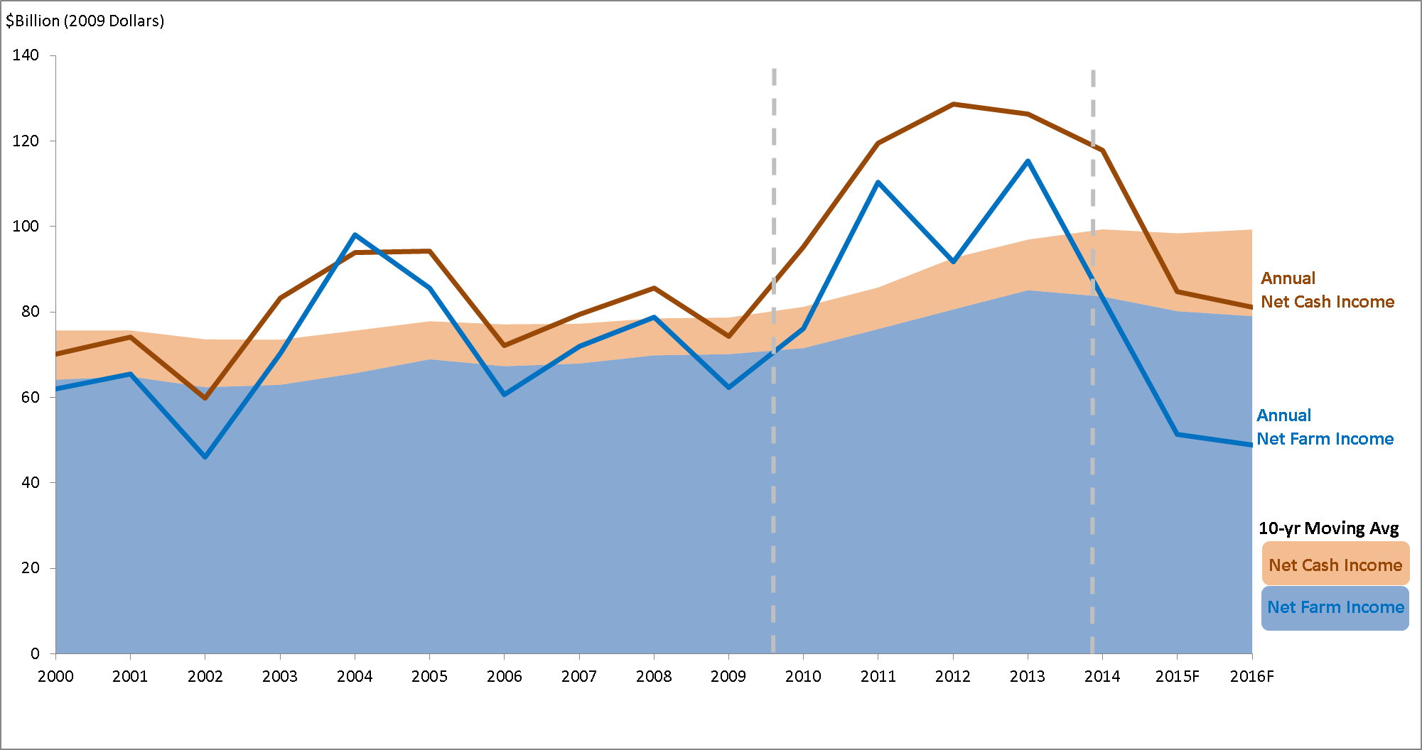
Net cash income and net farm income are two high-level, but comprehensive measures of farm sector profits. Net cash income reflects all cash income and expenses for the sector in a given year. Net farm income is a more complete measure of economic profitability that includes noncash income such as the value of inventory change, as well as noncash costs such as capital consumption. During the 20 years prior to 2010, both income measures increased modestly.
Footnotes: F=forecast. The GDP chain-type price index is used to convert
current dollars to real amounts (2009=100).
Source: USDA-ERS, 2015b.
Between 2009 and 2013, increasing commodity revenues combined with smaller expense increases led net cash and net farm income—and their 10-year moving averages—higher (Figure 1). Total commodity revenue grew by 38% over the 5-year period, driven largely by increases in commodity prices. The commodity revenue was helped by strong foreign demand for agricultural products, due in part to developing country growth and a relatively weak U.S. dollar combined with stable domestic demand bolstered by continued growth in the market for biofuels. Localized weather-related production disruptions also played a role in the increase in commodity revenue. The high prices that farmers received over this period outpaced the growth in production expenses. While input prices typically move in the same direction as commodity prices, they generally lag in adjustment. Zulauf (2014) finds it can take up to five years for the majority of the increase in crop prices to flow through to input prices.
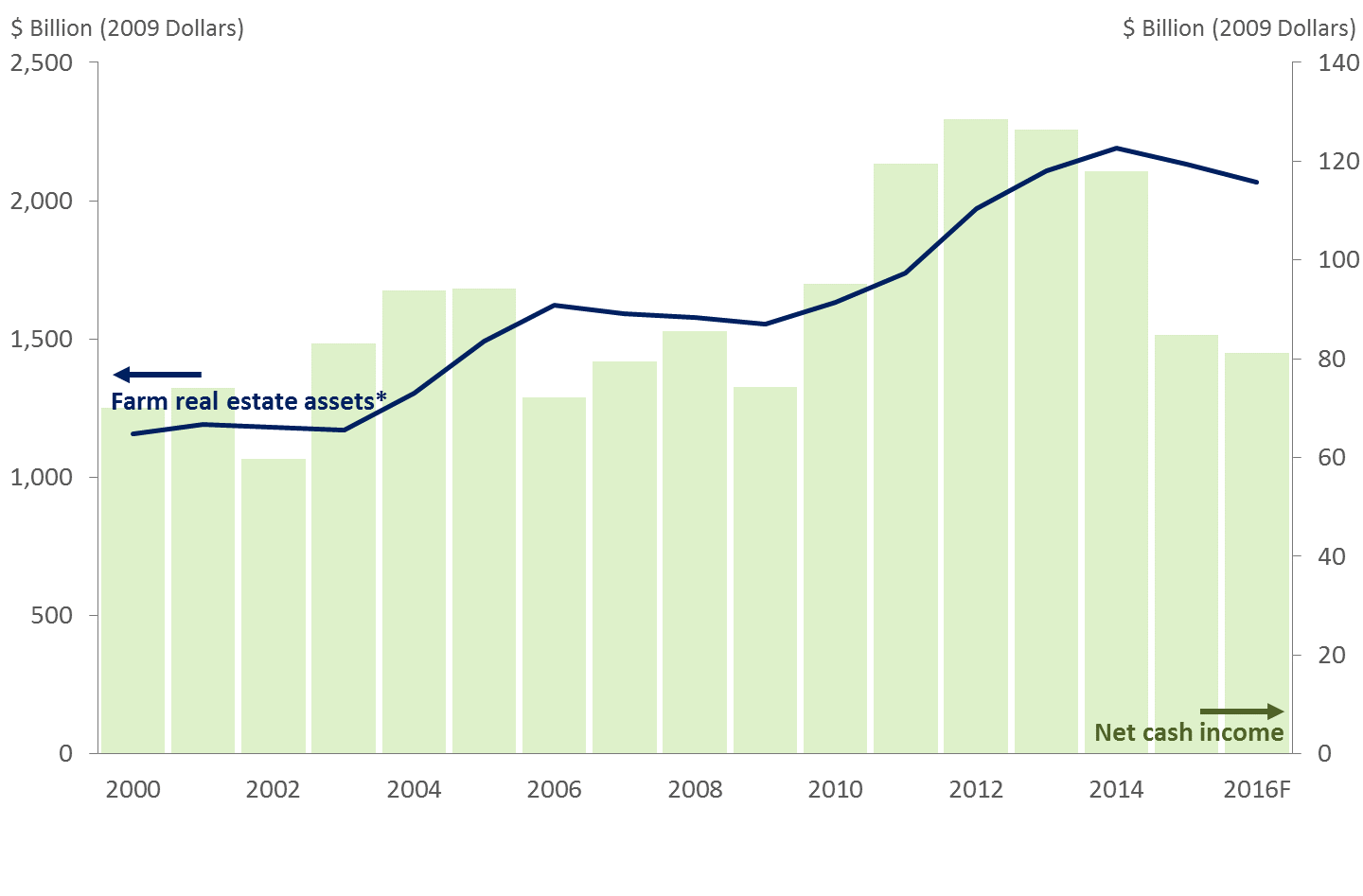
The factors supporting the rise in income also contributed to a strong sector balance sheet during this period. Historically, more than seven out of every ten dollars of total farm assets are attributable to real estate—including land and buildings—therefore increases in farm real estate values drive the growth in the value of total assets on the farm balance sheet. Between 2009 and 2013, increases in farm real estate represented $699 billion—or 87%—of the $808 billion change in total sector assets. The increases in farm real estate values followed the rise in income over this period (figure 2). From 2009 to 2013, the value of farm real estate assets increased at a 9.7% annual percentage rate (APR). By comparison, these asset values grew at a 5.8% APR between 2000 and 2009.
Footnotes: F=forecast. The GDP chain-type price index
is used to convert current dollars to real amounts
(2009=100).
Source: USDA-ERS, 2015b and USDA-NASS, 2015b
Footnote: All figures are in Billions ($).
Source: USDA-ERS, 2015b.
Between 2009 and 2013, the other side of the sector’s balance sheet—debt—rose only 17% ($47 billion). Rapidly increasing asset values and smaller increases in debt caused sector equity to rise by $761 billion.
Following the farm sector’s high income and rapid asset appreciation during the 2009-2013 period, net farm income and net cash farm income both fell modestly in 2014. USDA forecasts the decline to continue with a sharp decrease in 2015 and a third consecutive—though small—decline in 2016. Net farm income is expected to have declined 38% from 2014 to 2015, which would mark the largest year-over-year decrease since 1983. From 2014 to 2015, net cash farm income is projected to fall 27%, which would be the largest percentage decrease since the 1930’s. Both net farm income and net cash farm income are forecast to decline marginally in 2016, down 2.5% and 3%, respectively. Even though both measures are forecast to be well below their 10-year moving averages, and have declined sharply since 2013, the declines must be taken in context. In 2013 inflation-adjusted net farm income and net cash farm income were at or near their highest levels since 1973. Despite the large declines, the 2016 values for both income measures are in line with income levels prior to 2009, even after adjusting for inflation.
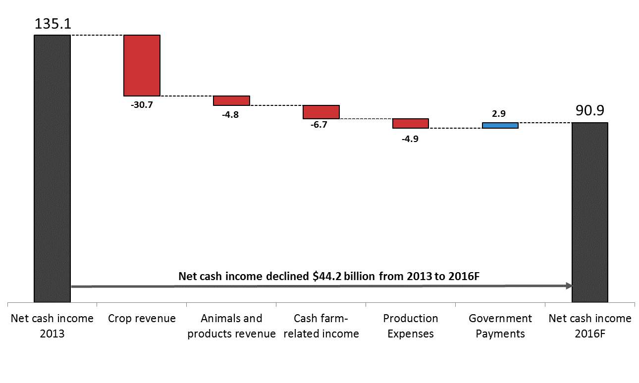
The decline in farm sector income was primarily driven by a significant drop in commodity revenue (Figure 3). In particular, lower crop revenue accounts for 86% of the forecasted decline in total commodity revenue, and 70% of the total decline in net cash income between 2013 to 2016. The drop in crop revenue has largely resulted from a broad-based decline in crop prices, rather than falling production. In particular, multiple years of record or near record corn and soybean harvests led prices downward for these commodities, which historically have represented more than 25% of the farm sector’s revenue. While small in comparison, animal and animal product revenues are also expected to decline by almost $5 billion between 2013 to 2016. Again, lower prices are the primary cause of the predicted decline.
In addition to the drop in revenue, expenses are expected to remain above 2013 levels. Total sector expenses increased almost 6% in 2014 and although they are forecast to fall by 3% and 1% in 2015 and 2016, respectively, they are still near their historic highs. As was the case when income was on the upswing from 2009-2013, input costs are expected to move in the same direction as commodity prices in 2015 and 2016, but adjustments in input costs lag changes in commodity prices, and are not expected to be of the same magnitude as the changes in commodity prices. Therefore, expected declines in sector expenses are not projected to fully compensate for falling revenues by 2016 and results in a decline in farm income.
Falling farm income is projected to impact the sector’s balance sheet in multiple ways. Year-end farm real estate values are expected to decline modestly in 2015 and 2016 following the trend in farm income. Lower commodity prices negatively impact the value of farm inventory assets by reducing the per-unit value of stored crops, animals and animal products. Combined, total farm sector asset values are expected to decline for the first time since 2009, falling 2.8% in 2015 and 1.6% in 2016. Prior to 2015 farm sector assets had only declined two other times since 2000, with each of the previous declines also coinciding with downturns in farm income.
The farm sector’s balance sheet also reflects a projected rise in farm debt use, in part due to reduced cash income. Even though it can eventually become more difficult to aquire debt if low levels of income are sustained for extended periods of time, lender data suggest the pace of nonreal estate borrowing—particularly operating loans—has increased markedly since 2013 (Kauffman, Cowley, and Clark, 2016). The impact of the expected decrease in farm assets in 2015 and 2016 and the increase in farm debt use since 2013, has negatively impacted the farm sector’s balance sheet relative to the 2009-2013 time period.
Source: USDA-ERS, 2015b.
Source: USDA-ERS, 2015b.
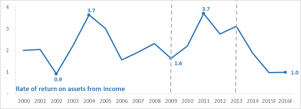
The increase in farm income and asset values over the 2009-2013 period was also reflected in improved measures of sector profitability such as the return on assets (ROA) ratio. The ROA is a measure of the income produced by the sector’s assets. Higher ROA values indicate the sector’s assets are generating more income signaling increased profitability. Not surprisingly, ROA increased from 2009 to 2013 (Figure 4a).
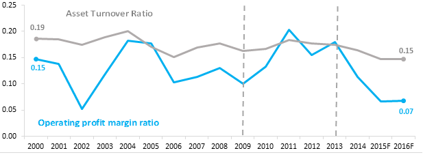
To get a better idea of what was driving profitability increases over this time period, it is possible to decompose ROA into how efficiently farm assets were used to generate output and the sector’s profit margin on that output (Figure 4b,). The asset turnover ratio measures the value of farm assets used to generate a dollar’s worth of output, and the operating profit margin ratio measures the income per dollar of output. From 2009-2013, the sector’s asset turnover ratio was relatively flat, at $0.18 of production per dollar of assets throughout the period. In contrast, the operating profit margin ratio rose sharply, increasing 80% to $0.17 of cash income per dollar of output. This suggests the primary factor driving the sector’s surging income and asset values was the rapid increases in profit margin seen during this time period. This further reinforces that changes in input prices tend to lag swings in commodity prices.
The farm sector’s ROA is expected to fall from a high of over 3% during 2009-2013 back down to 1% in 2015 and 2016. If realized this would represent the lowest sector ROA since 2002. The asset turnover ratio is expected to decline moderately relative to 2013. However, as was the case for the increase in ROA during the 2009-2013 period, changes in profitability drive the majority of the projected drop in ROA from 2013 to present. This again demonstrates what is seen in the farm income statement—the value of production has fallen significantly since 2013, while over the same period, farm sector expenses are forecast to have increased modestly. This squeeze on the top and bottom of the income statement drives down profitability, as illustrated by the expected 61% drop in operating profit margin ratio in 2016 compared to 2013.
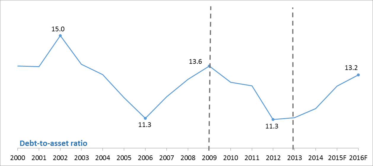
In addition to the sector’s profitability, the sector’s solvency risk—the risk of default from being unable to pay long-term obligations as they come due—a measure of the farm sector’s financial health. The debt-to-asset (D/A) ratio is one of the simplest measures of financial risk, conveying the portion of total farm assets that are financed by debt. Since a higher percentage of assets financed by debt results in less flexibility for the sector assets to cover potential financial liabilities, lower D/A ratios are generally preferable—lower percentage indicates less leverage and less risk. The farm sector’s D/A ratio improved during the 2009-2013 period due in part to the positive effect of increased income on asset values relative to debt levels.
Footnote: F= Forecast.
Source: USDA-ERS, 2015b.
Since spiking at over 22 during the 1980s farm financial crisis, the sector’s D/A ratio has trended lower, reaching a historical low in 2012. The D/A ratio has been increasing every year since 2012, and is forecast to continue increasing in 2015 and 2016 (Figure 5). The increasing D/A ratio—signaling an increase in financial leverage and therefore an increase in financial risk—reflects the impact of the large forecasted drop in farm income on the sector’s balance sheet. While the farm sector’s D/A ratio is expected to increase in 2015-2016, sector leverage remains low relative to historical trends. Only 13% of the value of farm sector assets are projected to be secured by debt in 2016, an amount substantially lower than the peak reached in the 1980s. Therefore, the sector as a whole appears relatively well insulated from risk associated with declining commodity prices, adverse weather, changing macroeconomic conditions, and others factors causing fluctuations in farm balance sheet values.
The sector-level trends reflect the economic performance of the farm economy as a whole. However, changes in sector-level income and total sector real estate asset values accrue to farm operators as well as other agricultural stakeholders, including nonoperator landowners. According to a new USDA survey—the 2014 Tenure, Ownership and Transition of Agricultural Land (TOTAL) survey—39% of land in farms (in the 48 contiguous States) was rented or leased. A portion (8% of land in farms) of this rented land was rented from other farm operators. However, the majority (31% of land in farms) of rented land was rented from non-operators. Therefore, both farm operators and non-operators benefit from, or are vulnerable to, changes in farm income and asset values.
Footnote: Excludes Alaska and Hawaii.
Source: USDA-ERS and USDA-NASS, 2015.
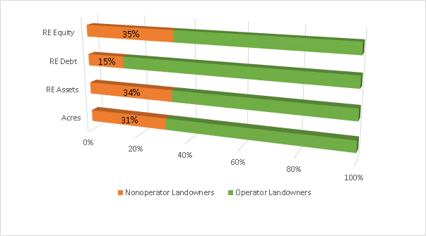
Non-operator landowners rented out 31% of all land in farms, which represented 34% of the sector’s value of real estate assets according to the 2014 TOTAL survey (Figure 6). In contrast, non-operator landowners hold a disproportionately low portion of sector debt—only 15%. As a result, non-operator landowners account for 35% of farm real estate equity.
The farm sector’s balance sheet nests the balance sheet of both operators and non-operator landlords. Because non-operators own a larger share of the sector’s real estate assets than real estate debt, the farm sector’s balance sheet may appear relatively stronger than if only the assets and debt owned by farm operations are examined. In addition, certain farms may use debt more aggressively than others, causing the sector balance sheet to mask heterogeneity among farms. Therefore, looking at the leverage for farm operations, and in particular farm businesses, may better illustrate the extent sector-level trends are reflected in the financial standing of individual farm operations.
Farm businesses— those farms with at least $350,000 in sales or farms with lower revenues where the operator’s primary occupation is farming—account for more than 90% of the sector’s production, and hold 71% of all farm assets and 80% of farm debt, according to the 2014 Agricultural Resource Management Survey (ARMS). Therefore, examining changes in the leverage position of farm businesses will provide a good gauge of how closely changes in the solvency risk for these operations compares to the total sector’s solvency risk, which includes non-operator landlords in addition to farm operators. Because farm businesses represent such a substantial portion of the farm sector, the change in the average farm business D/A ratios shows a similar pattern to that seen in the sector as a whole. After reaching a near record low of 9.3 in 2011, the average farm business D/A ratio has been increasing and is expected to be higher, at 13, in 2016. However, farm businesses, like the sector, have relatively low leverage on average.

Footnote: F= Forecast.
Source: USDA-ERS, 2015a.
Because farm businesses vary in the intensity of their debt use, using averages can hide growing risks among lower performing farms. In 2016, over 11% of farm businesses specializing in crop production are expected to have a D/A over 40, and nearly half of these farms are expected to have a D/A greater than 70 meaning that over 70% of their assets are financed by debt, indicating the operations are highly leveraged (Figure 7). Similarly, almost 9% of farm businesses specializing in animals and animal products are expected to have a D/A over 40 in 2016, while just over 3% are expected to have a D/A greater than 70. The share of farm businesses with high leverage is currently trending upward, but is still below the levels that prevailed in the late 1990’s when the data series began. However, in 2016 the share of crop farms with D/A ratios over 70 is expected to reach the second highest level since 1996. Because lending institutions consider D/A, among other financial ratios, to assess credit worthiness of farms, some of these highly leveraged farm businesses may have difficulty securing a loan. Additional years of declining income and asset values could also put these farms at risk of default.
Over a prosperous five-year period beginning in 2009, the U.S. farm sector’s income grew rapidly. From 2009 to 2013, increases in sector commodity revenues—due to increasing prices—outpaced sector expense increases, leading net income higher. Accordingly, the strength of the farm sector’s financial position also improved, highlighted by improvements in traditional financial indicators, such as the ROA and D/A ratios. However, after several years of strong performance, net farm and net cash income fell in 2014, and USDA forecasts both to decline sharply in 2015 and continue with a modest decline in 2016. As with the increase seen from 2009 to 2013, the decline in net income from 2014 to 2016 is driven by changes in sector commodity revenues, due largely to lower prices, outpacing changes in sector expenses. The income declines are expected to result in a modest reduction in farm sector assets, particularly real estate, and lead to an expansion in farm debt. While this means sector financial indicators are worsening relative to the 2009-2013 period, they remain at historically favorable levels. Nevertheless, the share of farms which are highly leveraged has increased since 2011, approaching 20-year highs. This is particularly the case for crop farm businesses which have seen a large reversal in commodity prices. Highly leveraged farm businesses are most vulnerable to additional financial stress in the near future if they experience negative shocks to their income or asset values. The extent to which these farm businesses and the sector as a whole show increasing signs of financial stress, will be shaped by any future declines in commodity prices, as well as how quickly and to what magnitude input prices respond to changing commodity prices. Therefore, the continued interaction between changes in agricultural commodity prices and the cost of inputs will have significant bearing on the financial well-being of U.S. farms in the years ahead.
Ifft, J., A. Novini, and K. Patrick. 2014. Debt Use by U.S Farm Businesses, 1992-2011. U.S. Department of Agriculture, Economic Research Service, Econ. Info. Bull. No. 122, April.
Kauffman, N., C. Cowley, and M. Clark. 2016. “Farm Loan Volumes Holding at High Levels.” Ag Finance Databook 1st Quarter Release, Fed. Reserve Bank of Kansas City, January.
U.S. Department of Agriculture, Economic Research Service (USDA-ERS). 2015a. “Agricultural and Resource Management Survey Farm Financial and Crop Production Practices.” Available online: http://www.ers.usda.gov/data-products/arms-farm-financial-and-crop-production-practices/questionnaires-and-manuals.aspx
U.S. Department of Agriculture, Economic Research Service (USDA-ERS). 2015b. “U.S. and State Farm Income and Wealth Statistics.” Available online: http://www.ers.usda.gov/topics/farm-economy/farm-sector-income-finances.aspx
U.S. Department of Agriculture, Economic Research Service (USDA-ERS) and U.S. Department of Agriculture, National Agricultural Statistics Service (USDA-NASS). 2015. “2014 Tenure, Ownership and Transition of Agricultural Land, August.” Available online: http://www.agcensus.usda.gov/Publications/TOTAL/
U.S. Department of Agriculture, National Agricultural Statistics Service (USDA-NASS). 2015a. Farms and Land in Farms 2014 Summary, Washington DC, February.
U.S. Department of Agriculture, National Agricultural Statistics Service (USDA-NASS). 2015b. Land Values 2015 Summary, Washington DC, August.
Zulauf, C., and N. Rettig. 2014. "U.S. Farm Input Price Dynamics, 1981-2013." Farmdoc Daily (4):221, Department of Agricultural and Consumer Economics, University of Illinois at Urbana-Champaign, November. Available online: http://farmdocdaily.illinois.edu/2014/11/us-farm-input-price-dynamics-1981-2013.html

